Solving SLAM with variational inference
19th September 2017, Taku Yoshioka
I started to working on robotics since this April, while I have made some contributions on the development of PyMC3, which is a probabilistic programming language. Thus, I think if PyMC3 can be applied to a problem of robotics. In this notebook, We will see how probabilistic programming can be applied to a problem of robotics, although it’s setting is very simple and not intended for real application.
Although single word “robotics” covers a lot of subfields of robotics research, here we will consider SLAM, which is the abbreviation for simultaneous localization and mapping. We can cast SLAM problem into Bayesian inference. We suppose that a car is moving on a map. The state of the car at time \(t\) is represented as a three dimensional vector \(\bf{s}_{t}\) of its 2-D location and the angle of its direction. Probabilistic models of SLAM problems can be written as \(p(\bf{M}, \bf{S}\mid\bf{Z},{\bf U})\), where \({\bf S}={\bf s}_{t=1:T}\), \({\bf M}\) denotes the map, \({\bf Z}\) denotes observations, and \({\bf U}={\bf u}_{t=1:T}\) denotes a sequence of control signals for the system. This equation means the posterior probability of car states and the map given observations.
A SLAM model
Specifically, we suppose a set of landmarks, which we considered as the map. It mean that \({\bf M}\) is a set of the locations of the landmarks: \({\bf m}_{j=1:M}\), where \(M\) is the number of the landmarks. However, the locations of the landmarks in a global coordinate are supposed to be unknown. Thus, we need to estimate thier locations from observations.
We also assume that the distance and the relative angle to each landmark from the car can be observed (\({\bf Z}\)), although there is a range of the measurements of distance and angle. It should be noted that the number of observations at each time step can vary.
We further assume that we know the sequence of control signals (\({\bf U}\)). Each signal consists of the velocity and stearing angle. The car move toward the current direction and the direction changes based on the stearing angle and the current velocity, which is a sipmle model of car movement.
Bayesian inference for SLAM
In the following, we will define the probabilistic model as \(p({\bf Z},{\bf S},{\bf M}\mid{\bf U})=p({\bf Z}|{\bf S},{\bf M})p({\bf S}|{\bf U})p({\bf M})\). \(p({\bf Z}|{\bf S},{\bf M})\) is referred to as observation model or likelihood. \(p({\bf S}|{\bf U})\) is the motion model. \(p({\bf M})\) is a prior distribution on the map (set of landmarks). Since we know control signals and the car movement model, we can estimate car location by accumlation of movements under the movement model. This accumlation process is involved to get \(p({\bf S}|{\bf U})\). This term is considered as a prior on \({\bf S}\). The prior distribution is modified based on the likelihood and more accurate estimation of \({\bf S}\) and \({\bf M}\) are obtained as its posterior.
Particle filter and extended Kalman filter (EKF) are commonly applied to infer \(p({\bf s}_{t=T},{\bf M}\mid{\bf s}_{t=1:(T-1)},{\bf Z},{\bf U})\). The former is a nonparametric method, while the later assumes a parametric model: Gaussian model with linealization around the current state. Inference of the states over time, \(p({\bf S},{\bf M}|{\bf Z},{\bf U})\) is referred to as a smoothing and is solved by extended Kalman smoother. Kalman filters requires to compute variance-covariance matrix of all states and landmark locations, thus does not scale the number of states and locations well.
PyMC3 supports variational inference, which approximates the true posterior by a parametric model. In addition, there is no need to write the code for doing probabilistic inference. It is sufficient for user to define the probabilistic model to be solved. This automated inference system is called automatic differentiation variational inference (ADVI). The most simple approximation of the true posterior is mean field: \(p({\bf S},{\bf M}\mid {\bf Z},{\bf U})\sim \prod_{t=1:T}q({\bf s}_{t})\prod_{j=1:M}q({\bf m}_{j})\). In this notebook, we use a mean-field model. It should be noted that PyMC3 also supports correlated posterior based on Stein gradiant variational inference or normalizing flows.
Contents of this notebook
This notebook consists of the three parts: simulation, SLAM model and inference. In simulation, artificial data is generated with a car model. In SLAM model, we define a Bayesian probabilistic model consisting of car motion and observation models with the help of PyMC3 syntax. Finally, posterior distribution of unknown random variables (\({\bf M}\) and \({\bf S}\)) are inferred automatically by using ADVI.
- Simulation
- Environment
- Run simulation
- SLAM Model
- Motion model
- Observation model
- Full model
- Inference
- ADVI
In [1]:
import sys
sys.path.insert(0, '/home/jovyan/work/git/github/pymc-devs/pymc3')
In [2]:
%matplotlib inline

import numpy as np
import pymc3 as pm
from pymc3 import Normal, Model
import matplotlib.pyplot as plt
import theano.tensor as tt
Simulation
Environment
Environment consists of a motion model, observation model and its parameters. The parameters includes:
- Landmark locations
- Initial car status
- Sequence of control signals
- Time difference for simulation
All parameters are stored in a dict.
In [3]:
n_timepoints = 40 # The number of time steps

env = {
    # Discritized time
    'n_timepoints': n_timepoints,

    # Landmark locations
    'landmark_locs': np.array([
        [-20.0, 20.0, 0.0, 0.0], # x-coord [m]
        [0.0, 0.0, -10.0, 30.0]  # y-coord [m]
    ]).T,

    # The initial state of the car
    'car_init': np.array([0., -5.0, 0.]), # x, y, angle

    # Control sequence
    'control': np.array([
        5.0 * np.ones(n_timepoints), # velocity [m/s]
        0.05 * np.pi * np.ones(n_timepoints)  # stearing angle [rad]
    ]).T,

    # Physical parameters
    'dt': 1.0, # time difference [s]
    'b': 2.0, # length of the car [m]

    # Sensor parameters
    'sensor_min_range': 1.0,  # 1.0 [m]
    'sensor_max_range': 50.0, # 50.0 [m]
    'sensor_min_angle': -0.3 * np.pi, # [rad]
    'sensor_max_angle': 0.3 * np.pi, # [rad]

    # Intrinsic noise in car movement
    'noise_move': np.array([0.1, 0.1, 0.1]), # ([m], [m], [rad])
    #'noise_move': np.array([0.4, 0.4, 0.02]), # ([m], [m], [rad])
}
The motion model transforms the current car state to the next one. It involves intrinsic noise which perturbates the car movement.
In [4]:
def simulate_movement(s, u, env, rng=None):
    dt, b = env['dt'], env['b']

    vdt = u[0] * dt
    s_ = np.stack((
        s[0] + vdt * np.cos(s[2] + u[1]),
        s[1] + vdt * np.sin(s[2] + u[1]),
        s[2] + vdt / b * np.sin(u[1])
    ))

    # Wrap angle (see https://stackoverflow.com/questions/15927755)
    s_[2] = (s_[2] + np.pi) % (2 * np.pi) - np.pi

    if rng is None:
        return s_
    else:
        return s_ + env['noise_move'] * rng.randn(3)
The observation model simulates range-bearing measurement, which
consists the distance and angle to landmarks from the current car
location. It should be noted that if a landmark is too far or too near
the car location, it is not able to be observed. These thresholds are
some variables in env.
In [5]:
def simulate_observation(s, env, rng):
    ms = env['landmark_locs']
    min_range = env['sensor_min_range']
    max_range = env['sensor_max_range']
    min_angle = env['sensor_min_angle']
    max_angle = env['sensor_max_angle']

    ds, ps, ixs = [], [], []

    for i in range(len(ms)):
        dx = ms[i][0] - s[0]
        dy = ms[i][1] - s[1]
        dist = np.sqrt(dx**2 + dy**2)
        angl = np.arctan2(dy, dx) - s[2]

        # Wrap angle (see https://stackoverflow.com/questions/15927755)
        angl = (angl + np.pi) % (2 * np.pi) - np.pi

        within_range = (min_range <= dist) and (dist <= max_range)
        within_angle = (min_angle <= angl) and (angl <= max_angle)

        # Add an observation
        if within_range and within_angle:
            noise_d = 0.01 * rng.randn(1)[0]
            noise_p = 0.01 * rng.randn(1)[0]
            # more realistic noise model
            # noise_d = dist / 10.0 * rng.randn(1)[0]
            # noise_p = 3.0 * np.pi / 180.0 * rng.randn(1)[0]

            d = dist + noise_d
            p = angl + noise_p

            ds.append(d)
            ps.append(p)
            ixs.append(i)
        else:
            pass

    if 0 < len(ds):
        return np.array([ds, ps]).T, np.array(ixs)
    else:
        return None, None
Run simulation
We are ready to run the simulation by using functions defined above. The function below simply applies the motion and observation models repeatedly.
In [6]:
def run_simulation(env):
    """Simulate car movement and range-bearing measurement under the given environment.

    Returned dict includes the following items:

    - ss: Car states. numpy.ndarray, shape=((n_timepoints + 1), 3).
    - ns: Series of the number of observed landmarks. numpy.ndarray, shape=(n_timepoints, 3).
    - zs: Series of observations. numpy.ndarray, shape=(n_obs_landmarks, 2).
    - ixs: Indices of the observed landmarks through the car movement. numpy.ndarray, shape=(n_obs_landmarks, 3).

    ss includes the initial car state.
    """
    rng = np.random.RandomState(0)
    us = env['control']
    dt = env['dt']

    rs = [env['car_init']] # odometry
    ss = [env['car_init']]
    ns = []
    zs = []
    ixs = []

    for i in range(n_timepoints):
        s = simulate_movement(ss[-1], us[i], env, rng)
        zs_, ixs_ = simulate_observation(s, env, rng)
        ss.append(s)

        r = simulate_movement(rs[-1], us[i], env)
        rs.append(r)

        if zs_ is None:
            ns.append(0)
        else:
            ns.append(len(ixs_))
            zs.append(zs_)
            ixs.append(ixs_)

    ss = np.vstack(ss[1:])
    rs = np.vstack(rs[1:])
    ns = np.stack(ns).reshape(-1)
    zs = np.concatenate(zs).reshape((-1, 2))
    ixs = np.concatenate(ixs).reshape(-1)

    return {
        'ss': ss,
        'rs': rs,
        'ns': ns,
        'zs': zs,
        'ixs': ixs
    }
In [7]:
def plot(env, result):
    n_timepoints = env['n_timepoints']

    # Landmarks
    ms = env['landmark_locs']
    plt.scatter(ms[0, 0], ms[0, 1], marker='*', color='r', s=200)
    plt.scatter(ms[1, 0], ms[1, 1], marker='*', color='g', s=200)
    plt.scatter(ms[2, 0], ms[2, 1], marker='*', color='b', s=200)
    plt.scatter(ms[3, 0], ms[3, 1], marker='*', color='c', s=200)

    if result is not None:
        ss = result['ss']
        rs = result['rs']
        zs = result['zs']
        ns = result['ns']
        ixs_ = [i * np.ones(ns[i], dtype='int') for i in range(n_timepoints) if 0 < ns[i]]
        ixs_ = np.concatenate(ixs_).reshape(-1)

        # Car locations
        plt.scatter(ss[:, 0], ss[:, 1], alpha=0.2)
        plt.plot(ss[:, 0], ss[:, 1], alpha=0.2)

        # Odometry
        plt.scatter(rs[:, 0], rs[:, 1], alpha=0.2, c='g')
        plt.plot(rs[:, 0], rs[:, 1], alpha=0.2, c='g')

        # Range-bearing measurements
        for i in range(len(zs)):
            s0 = ss[ixs_[i], 0]
            s1 = ss[ixs_[i], 1]
            e0 = s0 + zs[i, 0] * np.cos(zs[i, 1] + ss[ixs_[i], 2])
            e1 = s1 + zs[i, 0] * np.sin(zs[i, 1] + ss[ixs_[i], 2])
            plt.plot([s0, e0], [s1, e1], c='r', ls='--', alpha=0.5)

    plt.axes().set_aspect('equal', 'datalim')
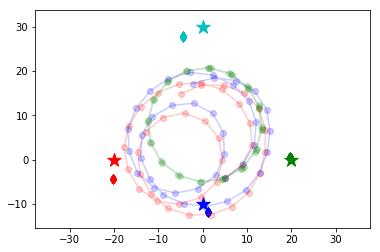
The below figure shows the car trajectory (blue circles), observations of landmarks (dotted red lines) and the noiseless trajectory (green circles). We see that the noiseless trajectory differs with the true trajectory. It is expected that the true trajectory is estimated accurately by combining the noiseless trajectory and the observations.
In [8]:
result = run_simulation(env)
plot(env, result)
SLAM probabilistic model
Motion model
In [9]:
def motion_model(s0, us, dt, b):
    """Add prior on the car states into the probabilistic model in the context.

    :param s0: The initial state of the car.
    :type s0: numpy.ndarray, shape=(3,)
    :param us: Control sequence.
    :type us: numpy.ndarray, shape=(n_timepoints, 3)
    :return: State variables for the car (random variables).
    :rtype: PyMC3 random variable class, shape=(n_timepoints, 3)
    """
    n_timepoints = len(us)

    def f(s, u):
        vdt = u[0] * dt
        return tt.stack((
            s[0] + vdt * tt.cos(s[2] + u[1]),
            s[1] + vdt * tt.sin(s[2] + u[1]),
            s[2] + vdt / b * tt.sin(u[1])
        ))

    s_prev = s0
    ss = []

    for i in range(n_timepoints):
        s = Normal(name=('s_%d' % (i + 1)), mu=f(s_prev, us[i, :]), sd=0.01, shape=(3,))
        ss.append(s)
        s_prev = s

    return tt.stack(ss)
Observation model
In [10]:
def obs_mean(ixs, ns, ss, ms, debug=False):
    """Returns the mean of observations.

    :param ixs: Indices of the observed landmarks through the car movement.
    :type ixs: numpy.ndarray, shape=(n_obs_landmarks,)
    :param ns: The number of observed landmarks at each time points.
    :type ns: numpy.ndarray, shape=(n_timepoints,)
    :param ss: State variables for the car (random variables).
    :type ss: PyMC3 random variable class, shape=(n_timepoints, 3)
    :param ms: State variables for the landmarks (random variables).
    :type ms: PyMC3 random variable class, shape=(n_landmarks, 3)

    ixs and ns must satisfy sum(ns) == len(ixs).
    """
    assert(ns.sum() == len(ixs))

    if debug:
        mod = np
    else:
        mod = tt

    ixs_ = np.concatenate([i * np.ones(n, dtype=int) for i, n in enumerate(ns) if 0 < n])
    dxs = ms[ixs, 0] - ss[ixs_, 0]
    dys = ms[ixs, 1] - ss[ixs_, 1]

    ranges_mean = mod.sqrt(dxs**2 + dys**2)
    angles_mean = mod.arctan2(dys, dxs) - ss[ixs_, 2]

    # Wrap angle (see https://stackoverflow.com/questions/15927755)
    angles_mean = (angles_mean + np.pi) % (2 * np.pi) - np.pi

    zs_mean = mod.stack((ranges_mean, angles_mean)).T

    return zs_mean

def observation_model(zs, ss, ms, ixs, ns):
    """Add observation model (likelihood function) into the probabilistic model in the context.

    :param zs: Range-bearing observations of the landmarks.
    :type zs: numpy.ndarray, shape=(n_obs_landmarks,)
    :param ss: State variables for the car (random variables).
    :type ss: PyMC3 random variable class, shape=(n_timepoints, 3)
    :param ms: State variables for the landmarks (random variables).
    :type ms: PyMC3 random variable class, shape=(n_landmarks, 3)
    :param ixs: Indices of the observed landmarks through the car movement.
    :type ixs: numpy.ndarray, shape=(n_obs_landmarks,)
    :param ns: The number of observed landmarks at each time points.
    :type ns: numpy.ndarray, shape=()

    ixs and ns must satisfy sum(ns) == len(ixs).
    """
    zs_mean = obs_mean(ixs, ns, ss, ms)
    Normal('zs', mu=zs_mean, sd=0.01, shape=zs.shape, observed=zs)
Full-model
We obtain the probabilistic model for this problem by combining the motion and observation models.
In [11]:
def slam_model(env, result):
    # Known variables: initial state, control signals, etc.
    s0 = env['car_init']
    us = env['control']
    n_landmarks = len(env['landmark_locs'])
    dt = env['dt']
    b = env['b']

    # Known variables: observations
    ns = result['ns']
    zs = result['zs']
    ixs = result['ixs']

    # SLAM model
    with Model() as model:
        ms = Normal(name='ms', mu=0, sd=100.0, shape=[n_landmarks, 2]) # p(m)
        ss = motion_model(s0, us, dt, b)                               # p(s|s_0, u)
        observation_model(zs, ss, ms, ixs, ns)                         # p(z|m, s)

    return model
The code for probabilistic inference can be implemented with three lines of code:
In [12]:
with slam_model(env, result) as model:
    inference = pm.ADVI()
    approx = pm.fit(n=200000, method=inference)
Average Loss = 1,879.1: 100%|██████████| 200000/200000 [07:05<00:00, 470.36it/s]
Finished [100%]: Average Loss = 1,879.2
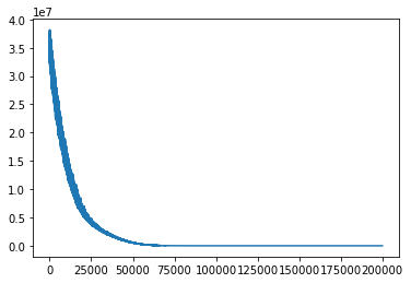
Here we see the negation of evidence lower bound (ELBO), which is the objective function used in ADVI.
In [13]:
plt.plot(inference.hist)
Out[13]:
[<matplotlib.lines.Line2D at 0x7f1c9b40aa20>]
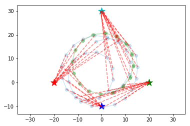
We can see that landmark locations (diamonds) and car locations (red circles) are estimated well.
In [14]:
trace = approx.sample(draws=100)
ms = trace['ms']

# Landmarks
# Inferred
plt.scatter(ms[:, 0, 0], ms[:, 0, 1], marker='d', c='r')
plt.scatter(ms[:, 1, 0], ms[:, 1, 1], marker='d', c='g')
plt.scatter(ms[:, 2, 0], ms[:, 2, 1], marker='d', c='b')
plt.scatter(ms[:, 3, 0], ms[:, 3, 1], marker='d', c='c')

# True
ms = env['landmark_locs']
plt.scatter(ms[0, 0], ms[0, 1], marker='*', color='r', s=200)
plt.scatter(ms[1, 0], ms[1, 1], marker='*', color='g', s=200)
plt.scatter(ms[2, 0], ms[2, 1], marker='*', color='b', s=200)
plt.scatter(ms[3, 0], ms[3, 1], marker='*', color='c', s=200)

# Car locations
# Inferred
ss = [trace[('s_%d' % i)].reshape(-1, 3).mean(axis=0) for i in range(1, n_timepoints + 1)]
ss = np.vstack(ss)
plt.scatter(ss[:, 0], ss[:, 1], alpha=0.2, c='r')
plt.plot(ss[:, 0], ss[:, 1], alpha=0.2, c='r')

# True
ss = result['ss']
plt.scatter(ss[:, 0], ss[:, 1], alpha=0.2, c='b')
plt.plot(ss[:, 0], ss[:, 1], alpha=0.2, c='b')

# Noiseless
rs = result['rs']
plt.scatter(rs[:, 0], rs[:, 1], alpha=0.2, c='g')
plt.plot(rs[:, 0], rs[:, 1], alpha=0.2, c='g')

plt.axes().set_aspect('equal', 'datalim')